Ranking without Duplicating Ranks

Preston Murphy · 08/28/20

I used the RANKEQ function for the first time recently and realized that any identical values will have the same rank. It will skip however many duplicates you had in the ranking numbers, so you may have a ranking scheme that looks like 1, 2, 3, 3, 3, 6, 7, 7, 9, 9.

This may be useful in some situations but it is actually problematic in other situations. Let's say I am searching for the top 10 values in my set. I will not find a value for 4, 5, 8, or 10. This will of course be frustrating if I want to simply plot the top 10 values from my data set.

I have created the following formula to ignore duplicates and simply increment the rank of any duplicates by 1. This means any duplicates will have an arbitrary ranking to each other.

In this formula, "A" is the column being ranked.

RANK=RANKEQ(A@row, A:A) + COUNTIF(A$1:A@row, RANKEQ(@cell, A:A) = RANKEQ(A@row, A:A)) - 1

Hopefully this helps someone!

Genevieve P. · 08/31/20

Hi@Preston Murphy

Thank you for sharing your solution with the Community!

Jeff Reisman · 01/19/21

@Preston Murphy

Thank you so much for this formula! It was a life saver. I used it as the basis for getting rankings based on multiple criteria. I hope the below can add on to your solution to help the next person with an issue similar to mine:

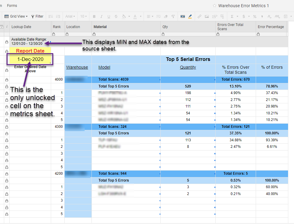
I have a sheet that gets re-populated each month with scan error data from three different warehouses, for each day of the month. Each row lists the date, the warehouse number, the model number, and how many scan errors were recorded. I needed to be able to find the top 5 models with the most scan errors for each warehouse, for each day. So 12/1/2020 would have a top 5 for Warehouse 4000, top 5 for Warehouse 4200, and top 5 for Warehouse 4300. I needed to be able to display these on a metrics sheet, where the user selects the date, and the system displays the Top 5 data for that date for each warehouse.

I was able to get a ranking for each date for each warehouse based on that criteria, but of course I had duplicate rankings. When I tried your formula, trying to embed the criteria into the RANKEQ formulas within the COUNTIF kept returning a #NESTED CRITERIA error. So frustrating!

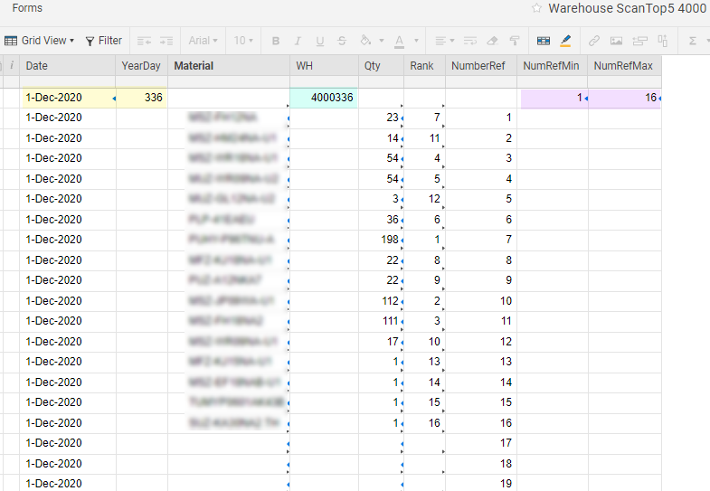
In my data table I have columns for Date (Date), Model # (Material), # of scan errors (Qty,) Rank (Rank) and one for Warehouse number joined to the day of the year based on the Date column (WH-Day). The WH-Day column combines the warehouse number and date into one field to identify all rows for a given warehouse on a given day. I have another column called Number, which is just a column of ascending numbers counting up from 1, going up to 400 (about as many data rows as I would have for a given month.)

=RANKEQ(Qty@row, COLLECT(Qty:Qty, [WH-Day]:[WH-Day], [WH-Day]@row), 0) + COUNTIF(Qty$1:Qty@row, RANKEQ(@cell, COLLECT(Qty:Qty, [WH-Day]:[WH-Day], [WH-Day]@row), 0) = RANKEQ(Qty@row, COLLECT(Qty:Qty, [WH-Day]:[WH-Day], [WH-Day]@row), 0)) - 1

This resulted in the #NESTED CRITERIA error. I tried various changes to the criteria, and either got #UNPARSEABLE or #INVALID DATA TYPE. The individual pieces of the above worked, until I had the entire COUNTIF piece by itself, then the nested criteria error.

What I ended up doing was creating helper sheets for each of the three warehouses. My source data is sorted by Date ascending, and then by Warehouse number ascending. For a given date, each warehouse's rows are in a contiguous range of the Number column.

In my helper sheets I have the following:

The [Date]1 cell links in from my metrics sheet (the user input to select date.) I get theYearDayvalue (=IF(YEARDAY(Date@row) < 10, "00", IF(YEARDAY(Date@row) < 100, "0")) + YEARDAY(Date@row)) and in theWHcolumn I join the warehouse number to the YearDay value (=VALUE(JOIN("4000" + YearDay@row)))

Using MIN and MAX I pull the beginning Number and ending Number for the WH value into theNumRefMinandNumRefMaxcolumns of Row 1:

=MIN(COLLECT({Warehouse Scan Error Data Number}, {Warehouse Scan Error Data WH-Day}, =WH@row))

I grab theMaterialvalue that matches theNumberRefvalue, provided theNumberRefis <= toNumRefMax:

=IF(NumberRef@row < VALUE(NumRefMax1 + 1), INDEX({Warehouse Scan Error Data Mat}, MATCH(NumberRef@row, {Warehouse Scan Error Data Number}, 0), 1), "")

I get theQtyvalue using the same criteria. Using IF allows me to avoid #NO MATCH or other errors when there is no matching value.

Once I have theMaterialandQtyvalues that are only for this warehouse on this day, I can use Preston's formula to get my rankings without duplicates! Again, I use an IF to avoid error values in any cells.

=IF(Qty@row > 0,RANKEQ(Qty@row, Qty:Qty) + COUNTIF(Qty$2:Qty@row, RANKEQ(@cell, Qty:Qty) = RANKEQ(Qty@row, Qty:Qty)) - 1, "")

With separate helper sheets for each warehouse, I can pull data onto my metrics sheet that gives me the correct rankings and values I need. User selects a valid date, hits save, and data updates in a few seconds (flashing in blue as the cells update.)

Preston Murphy · 01/21/21

@JReisman27

Wow!! I am really glad this helped! It seems you are really pushing Smartsheet to its limit, doing some advanced stuff here. Thanks for sharing!

TJones Hoshizaki · 05/03/21

Is there a way to do this without using an @cell in the formula? I am trying to right this on a sheet that I need to be able to convert to a Column Formula and @cell is not permitted for Column formulas?

Lindsay Whitbread · 05/27/21

A rank without duplicates is often referred to as a "Dense Rank".

I created this formula to make dense ranks. It needs a helper formula that contains the "Sparse" rank that RANKEQ provides.

Conceptually, you create a sparse rank with RANKEQ, then you RANK the Sparse Rank to create a Dense Rank...and then you map the correct Dense Rank to each of the Sparse Ranks.

In this example I rank the smallest value to the number 1 rank.

Helper column, which I called "Item Sparse Rank":

=IFERROR(RANKEQ([Item Value]@row, [Item Value]:[Item Value], 1), "")

Make that a column formula

Then you make your dense rank:

=IFERROR(RANKEQ([Item Sparse Rank]@row, DISTINCT([Item Sparse Rank]:[Item Sparse Rank]), 1), "")

And make that a column formula too. Now, I've adjusted these formula from my own to make it generic so let me know if they don't actually work.

Cheers,

Lindsay

Lewis Waters · 06/10/21

A rank without duplicates is often referred to as a "Dense Rank".<\/p>

I created this formula to make dense ranks. It needs a helper formula that contains the "Sparse" rank that RANKEQ provides.<\/p>

Conceptually, you create a sparse rank with RANKEQ, then you RANK the Sparse Rank to create a Dense Rank...and then you map the correct Dense Rank to each of the Sparse Ranks.<\/p>

In this example I rank the smallest value to the number 1 rank.<\/p>

Helper column, which I called "Item Sparse Rank":<\/p>

=IFERROR(RANKEQ([Item Value]@row, [Item Value]:[Item Value], 1), "")<\/p>

Make that a column formula<\/p>

Then you make your dense rank:<\/p>

=IFERROR(RANKEQ([Item Sparse Rank]@row, DISTINCT([Item Sparse Rank]:[Item Sparse Rank]), 1), "")<\/p>

And make that a column formula too. Now, I've adjusted these formula from my own to make it generic so let me know if they don't actually work.<\/p>

Cheers,<\/p>

Lindsay<\/p>","bodyRaw":"[{\"insert\":\"A rank without duplicates is often referred to as a \\\"Dense Rank\\\".\\nI created this formula to make dense ranks. It needs a helper formula that contains the \\\"Sparse\\\" rank that RANKEQ provides.\\nConceptually, you create a sparse rank with RANKEQ, then you RANK the Sparse Rank to create a Dense Rank...and then you map the correct Dense Rank to each of the Sparse Ranks.\\nIn this example I rank the smallest value to the number 1 rank.\\nHelper column, which I called \\\"Item Sparse Rank\\\":\\n=IFERROR(RANKEQ([Item Value]@row, [Item Value]:[Item Value], 1), \\\"\\\")\\nMake that a column formula\\nThen you make your dense rank:\\n=IFERROR(RANKEQ([Item Sparse Rank]@row, DISTINCT([Item Sparse Rank]:[Item Sparse Rank]), 1), \\\"\\\")\\nAnd make that a column formula too. Now, I've adjusted these formula from my own to make it generic so let me know if they don't actually work.\\n\\nCheers,\\nLindsay\\n\\n\"}]","format":"rich","dateInserted":"2021-05-27T12:57:46+00:00","insertUser":{"userID":127442,"name":"Lindsay Whitbread","title":"","url":"https:\/\/community.smartsheet.com\/profile\/Lindsay%20Whitbread","photoUrl":"https:\/\/aws.smartsheet.com\/storageProxy\/image\/images\/u!1!H-jC307v_hQ!5OfDeX66Zjw!fwqmUy9Jz6t","dateLastActive":"2023-08-26T11:30:59+00:00","banned":0,"punished":0,"private":false,"label":"✭✭✭"},"displayOptions":{"showUserLabel":false,"showCompactUserInfo":true,"showDiscussionLink":false,"showPostLink":false,"showCategoryLink":false,"renderFullContent":false,"expandByDefault":false},"url":"https:\/\/community.smartsheet.com\/discussion\/comment\/293099#Comment_293099","embedType":"quote"}"> https://community.smartsheet.com/discussion/comment/293099#Comment_293099

Hi Lindsay,

This gives me an INVALID DATA TYPE in the Dense rank field. Any ideas?

Lewis Waters · 06/10/21

Preston's solution is great, but really what I would love is duplicates to have the same ranking AND ranks not be skipped. i.e

A 1

B2

C3

D4

Lewis Waters · 06/10/21

https:\/\/community.smartsheet.com\/discussion\/comment\/293099#Comment_293099<\/a><\/p>

Hi Lindsay,<\/p>

This gives me an INVALID DATA TYPE in the Dense rank field. Any ideas?<\/p>","bodyRaw":"[{\"insert\":\"https:\\\/\\\/community.smartsheet.com\\\/discussion\\\/comment\\\/293099#Comment_293099\",\"attributes\":{\"link\":\"https:\\\/\\\/community.smartsheet.com\\\/discussion\\\/comment\\\/293099#Comment_293099\"}},{\"insert\":\"\\n\"},{\"insert\":\"Hi Lindsay,\\nThis gives me an INVALID DATA TYPE in the Dense rank field. Any ideas?\\n\"}]","format":"rich","dateInserted":"2021-06-10T12:11:37+00:00","insertUser":{"userID":120362,"name":"Lewis Waters","url":"https:\/\/community.smartsheet.com\/profile\/Lewis%20Waters","photoUrl":"https:\/\/us.v-cdn.net\/6031209\/uploads\/defaultavatar\/nWRMFRX6I99I6.jpg","dateLastActive":"2021-11-19T12:18:33+00:00","banned":0,"punished":0,"private":false,"label":"✭✭✭"},"displayOptions":{"showUserLabel":false,"showCompactUserInfo":true,"showDiscussionLink":false,"showPostLink":false,"showCategoryLink":false,"renderFullContent":false,"expandByDefault":false},"url":"https:\/\/community.smartsheet.com\/discussion\/comment\/294480#Comment_294480","embedType":"quote"}"> https://community.smartsheet.com/discussion/comment/294480#Comment_294480

Ok so when I use =value on the sparse rank it seems to do the trick!

MAshfield · 11/04/21

@Lewis WatersHi Lewis, could you please explain how you used the =VALUE to avoid the #INVALID DATA TYPE error?

Devin Lee · 11/26/21

Here is alterative that deals with blank cells in the ranking.

=IF(A@row = "", "", RANKEQ(A@row, A:A) + COUNTIFS(A$1:A@row, A@row <> "", A$1:A@row, RANKEQ(@cell, A:A) = RANKEQ(A@row, A:A)) - 1)

Kelly Moore · 03/12/22

Hey

One more build that allows the formula to eliminate blanks and be a column formula. One must add the system-generated auto-number column [Row ID] as a helper column (which could be hidden, if desired). This formula assumes that rows are being inserted at the bottom of the sheet.

-Kelly

= RANKEQ (A@row: A) +条件统计(一个,ISNUMBER (@cell), [Row ID]:[Row ID], <=[Row ID]@row, A:A, RANKEQ(@cell, A:A) = RANKEQ(A@row, A:A)) - 1)

Ranking without Duplicating Ranks

Comments

Categories